Abstract

Computer vision technologies, exclusively the deep convolutional neural network, have been quickly advanced in recent years. It is auspicious to use the state-of-art computer vision techniques to support people with eyesight loss. Images are a vital source of data and information in the up-to-date sciences. The practice of image-processing methods takes outstanding conjugation for the study of images. Today, many of the support systems installed for visually impaired people are mostly made for a single drive. Be it direction finding, object detection, or distance remarking. Also, most of the installed support systems use indoor navigation which needs a pre-knowledge of the situation. These help systems often flop to help visually impaired individuals in the unaccustomed scenario. In this paper, we suggest a support system established using object detection to direct an individual without dashing into an item. This project attempts to convert the visual world into the audio world with the potential to notify blind people objects. In my project, we figure a real-time object detection with the goal of notifying the user about nearby object. With this structure, we built a multi feature, high correctness directional support system by processing the image and performing calculation using image processing to help the visually impaired individuals in their daily life by navigating them smoothly to their looked-for destination and to read the data from the image with the help of image processing.

Chapter 1

Introduction

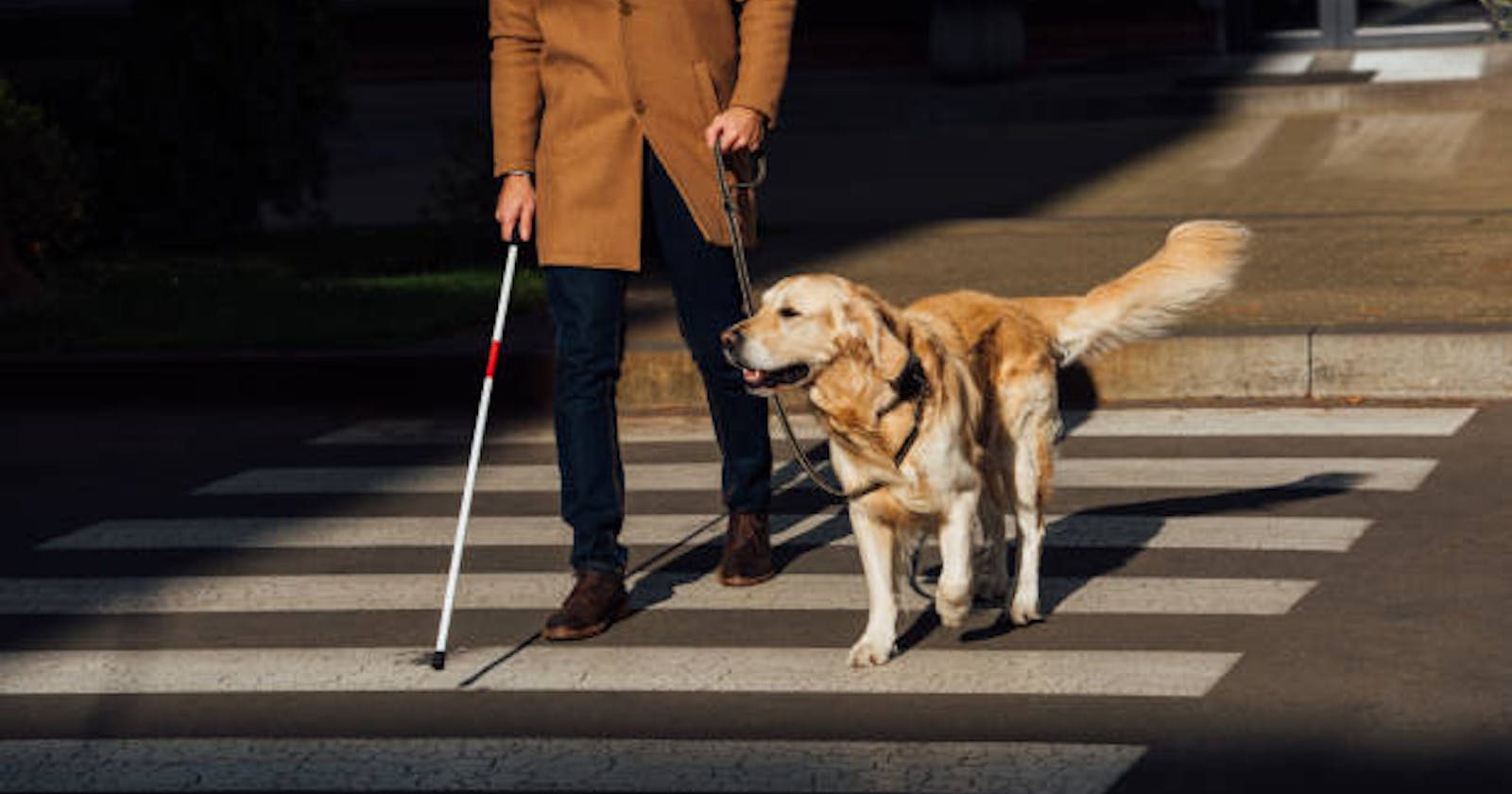
Mobility is one of the main problems bump into by the blind in their daily life. Imagine how is the life of an unsighted person, their life is full of risk, they can't even walk alone through a busy street or through a park. They continuously need some aid from others. In this project, we want to explore the opportunity of using the hearing sense to realize visual objects.

1.1 Motivation

Images are an important source of data and information. The use of image-processing techniques have outstanding implications for the analysis and operations. By using this, mine main motive is, to lower the sorrow and struggle level of the blind people.

1.2 Research Objective

We want to help blind travelers for a confident and independent movement. By my project, one can easily detect the object name and hear it. We want to Understand the practical applications with tremendous future possibilities and want to find out the suitable machine learning technique that is computationally efficient as well as accurate for the recognition of the image.

1.3 Research Contribution

The main contribution of the research is to the blind people for their movement. Previous studies can also detect the obstacle but the technology is from the ancient time, and their system is also time consuming. That’s why we try to build a better option for them. It is an unpublished work. So, we make a system and apply an appropriate algorithm for better output.

1.4 Organization of Thesis

The residual of the chapters of this thesis are arranging in the following ways: Chapter 2 summarizes the related works of blind aid system, what kind of Several approaches are following to build an assistance for the blind people. Here also what types of objects detection models and complexed microprocessor system were used to solve this problem were discussed. Chapter 3 reviews the algorithm and describes the CNN and Faster RCNN. In this chapter we have a brief description how my system works. In my thesis, we used COCO dataset having 100 classes for my research. This chapter also describes the model of my convolutional neural networks and methods in detail Chapter 4 describes the methodology of our system. This section provides brief algorithm information from the disciplines contributing to this thesis: Finding an effective pathway for blind people using image classification and voice Command. First presented details of Convolution Neural Network. Next introduced are topics related to Convolution Neural Network: Convolution layer, Stride, Padding Non-Linearity (ReLU), Pooling Layer, Fully Connected Layer. Finally covered with a brief description of Faster RCNN. Chapter 5 analyzes the experimental results which are found in the thesis. This section describes and analyzes the results we got from my experiments. At first, we investigate the effects of depth-wise convolutions and the option of contraction by decreasing the length of the network rather than the number of layers. Then show the trade-offs of decreasing the network based on the two hyper-parameters, width and resolution multiplier, and compare the results to some popular models. Chapter 6 discusses some future works and conclusions about blind aid system that can be implemented in the future. This chapter summarizes the whole research in several words describing the problem domain, previous researches, my contribution, experimental analysis and the outcomes of this research. Moreover, we have provided a brief study about the future scopes of this research. In this chapter, we try to present the importance of my system. We also try to introduce why we have selected this and the importance of my thesis. Here we discussed research objectives, research contribution and thesis organization to conclude the chapter.

Chapter 2

Related Work

Several approaches are following to build an assistance for the blind people. Many objects detection models and complexed microprocessor system were used to solve this problem. Microcontroller LPC2148, PIC 16F876, ultrasonic sensors were used previously but in modern literature, there are neural networks, especially convolutional neural networks, used to classify objects from images.

2.1 Microcontroller Based Model

A microcontroller is a reduced coordinated circuit intended to administer a particular activity in an installed framework. An ordinary microcontroller incorporates a processor, memory and info/yield (I/O) peripherals on a solitary chip. 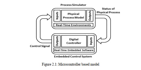Here and there alluded to as an installed regulator or microcontroller unit (MCU), microcontrollers are found in vehicles, robots, office machines, clinical gadgets, portable radio handsets, candy machines and home apparatuses, among different gadgets. They are basically basic smaller than usual (PCs) intended to control little highlights of a bigger part, without a perplexing front-end working framework (OS).5 In [3], they used Optical Character Recognition (OCR) technology but focused only for text reading. By using the system blind only will be able to read text characters. TTS feature can also read out the words. The system is suitable for an indoor situation only. In [21], they used an ultrasonic sensor and their system gives audio instructions for guidance.The authors of [22] used a microcontroller in their project. The model was PIC 16F876. It was embedded on an ultrasonic cane to detect any obstacle. In [23], It contains a laptop, a tracking chip, GPS sensors, 4 cameras and headphones. The LPC2148 microcontroller was there. The software modules they used are listed below:

• Embedded C
• Keil IDE
• Uc-Flash

A microcontroller is implanted within a framework to control a solitary capacity in a gadget. It does this by deciphering information it gets from its I/O peripherals utilizing its focal processor. The transitory data that the microcontroller gets is put away in its information memory, where the processor gets to it and utilizations directions put away in its program memory to unravel and apply the approaching information. It then, at that point, utilizes its I/O peripherals to impart and establish the proper activity. Microcontrollers are utilized in a wide exhibit of frameworks and gadgets. Gadgets regularly use various microcontrollers that cooperate inside the gadget to deal with their individual undertakings. For instance, a vehicle may have numerous microcontrollers that control different individual frameworks inside, for example, the stopping automation, footing control, fuel infusion, or suspension control. All the microcontrollers speak with one another to illuminate the right activities. Some may speak with a more intricate focal PC inside the vehicle, and others may just speak with other microcontrollers. They send and get information utilizing their I/O peripherals and cycle that information to play out their assigned undertakings.

2.2 Deep Learning-Based Model

Deep learning is a subset of AI, which is basically a neural organization with at least three layers. These neural organizations endeavor to mimic the conduct of the human cerebrum—though a long way from coordinating with its capacity—permitting it to "learn" from a lot of information. While a neural organization with a solitary layer can in any case make inexact expectations, extra secret layers can assist with advancing and refine for exactness. Deep learning drives numerous man-made consciousness (AI) applications and administrations that further develop automation, performing logical and actual undertakings without human intercession. Profound learning innovation lies behind regular items and administrations (like computerized aides, voice-empowered TV controllers, and charge card extortion discovery) just as arising advancements (like self-driving vehicles). 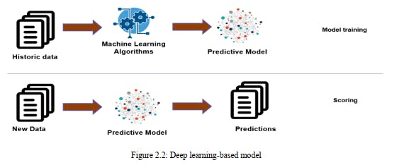Deep learning is a portion of machine learning. It is mainly a subset of machine learning. It works with neural networks. Deep learning wants to represent human brains virtually using neural networks. Deep learning has two models. These are:

• Supervised Models: Supervised learning model is a part of deep learning and a subcategory of machine learning. In this model, it labeled datasets to train algorithms. It classifies data and predicts outcomes accurately.
• Unsupervised Models: Unsupervised learning model is a part of deep learning. It is also known as an unsupervised machine learning model. This unlabeled model data sets to train algorithms

2.2.1 Different Types of Supervised Learning:

• Classic Neural Networks: Classic neural networks work as computer vision. It makes the computer process and understands images. It can process a huge number of images at a time. It is a supervised learning model.

• Convolutional Neural Networks (CNNs): These can scan images fast and make a better output. It can scan a whole image at a time. It automatically detects the important features without any human supervision.

• Recurrent Neural Networks (RNNs): A recurrent neural network is a type of supervised learning and artificial neural network. It uses sequential data. These neural networks are used for ordinal or temporal problems. It stimulates neuron activity in the human brain.

2.2.2 Different Types of Unsupervised Model:

• Self-Organizing Maps (SOM): A self-organizing map (SOM) is an unsupervised machine learning technique used to produce a low-dimensional (typically two-dimensional) representation of a higher dimensional data set while preserving the topological structure of the data. A SOM is a type of artificial neural network but is trained using competitive learning rather than the error-correction learning used by other artificial neural networks.

• Boltzmann Machines: A Boltzmann machine is a recurrent neural network in which nodes make binary decisions with some bias. Boltzmann machines can be strung together to create more sophisticated systems such as deep belief networks. A Boltzmann machine is also known as a stochastic Hopfield network with hidden units. Boltzmann machines are used to solve two quite different computational problems.

• Auto Encoders: An auto-encoder is a type of artificial neural network used to learn efficient coding of unlabeled data. They work by compressing the input into a latent space representation and reconstructing the output from this representation. An autoencoder consists of 3 components: encoder, code, and decoder. The encoder compresses the input and produces the code, and the decoder then reconstructs the information using this code.

In this chapter, we have tried to present the different types of models which are used in image recognition. we describe about microcontroller-based models, Deep learning models also. We also describe about the types of Deep learning models we use this of model for my research purpose.

Chapter 3

Methodology

In this section, we have a brief description of how my system works. In my thesis, we used the COCO dataset having 100 classes for my research. This chapter describes the model of my convolutional neural networks and methods in detail. The methodology is described in figure 3.1.

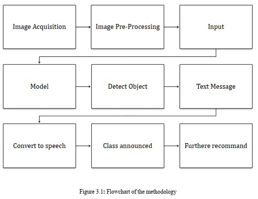
3.1 Methodologies Description

Methodology means the process we follow to build up my project. We follow some steps. These are given below:

3.1.1 Image Acquisition

A picture can be characterized as a 2-D capacity f(x,y) where (x,y) is co-ordinate in two dimensional space and f is the power of that co-ordinate. Every co-ordinate position is called as pixel. Pixel is the littlest unit of the picture it is likewise called as picture component. So computerized pictures are made out of pixels, every pixel addresses the shading (dark level for high contrast pictures) at a solitary point in the picture. Pixel resembles little speck of specific tone. A computerized picture is a rectangular cluster of pixels additionally called as Bitmap. According to the perspective of photography the computerized pictures are of two sorts:

• Black and white Images

• Color Images

The overall point of Image Acquisition is to change an optical picture (Real World Data) into a variety of mathematical information which could be subsequently controlled on a PC, before any video or picture preparing can initiate a picture should be caught by camera and changed over into a sensible element. The Image Acquisition measure comprises of three stages: -

• Optical system which centers the energy

• Energy reflected from the targeted object

Picture securing in picture handling can be comprehensively characterized as the activity of recovering a picture from some source, generally an equipment-based source, so it very well may be gone through whatever cycles need to happen thereafter. Performing picture procurement in picture handling is consistently the initial phase in the work process grouping in light of the fact that, without a picture, no handling is conceivable. The picture that is procured is totally natural and is the consequence of whatever equipment was utilized to produce it, which can be vital in certain fields to have a steady standard from which to work. One of the definitive-objective of this cycle is to have a wellspring of information that works inside such controlled and estimated rules that a similar picture can, in case important, be almost impeccably replicated under similar conditions so peculiar variables are simpler to find and take out. Contingent upon the field of work, a central point associated with picture securing in picture handling once in a while is the underlying arrangement and long-haul support of the equipment used to catch the pictures. The genuine equipment gadget can be anything from a work area scanner to an enormous optical telescope. Assuming the equipment isn't as expected arranged and adjusted, visual relics can be delivered that can entangle the picture handling. Inappropriately arranged equipment likewise may give pictures that are of such bad quality that they can't be rescued even with broad handling. These components are fundamental to specific regions, for example, similar picture handling, which searches for explicit contrasts between picture sets. One of the types of picture securing in picture handling is known as constant picture obtaining. This normally includes recovering pictures from a source that is naturally catching pictures. Ongoing picture procurement makes a flood of documents that can be consequently handled, lined for later work, or sewed into a solitary media design. One normal innovation that is utilized with ongoing picture handling is known as foundation picture procurement, which depicts both programming and equipment that can rapidly safeguard the pictures flooding into a framework. There are some best in class techniques for picture securing in picture handling that really utilize tweaked equipment. Three-dimensional (3D) picture procurement is one of these strategies. This can require the utilization of at least two cameras that have been adjusted at exactly portrays focuses around an objective, shaping a grouping of pictures that can be adjusted to cause a 3D or stereoscopic situation, or to quantify distances. A few satellites utilize 3D picture securing procedures to construct exact models of various surfaces. A sensor which calculates the total energy. Picture Acquisition is accomplished by appropriate camera. We utilize various cameras for various application. On the off chance that we need a x-beam picture, we utilize a camera (film) that is touchy to x-beam. Assuming we need infra-red picture, we use camera which are delicate to infrared radiation. For typical pictures (family pictures and so forth) we use cameras which are delicate to visual range. Picture Acquisition is the initial phase in any picture preparing framework.

3.1.2 Image Acquisition Model

The pictures are created by blend of a brightening source and the reflection or ingestion of the energy by the components of scene being imaged. Brightening might be begun by radar, infrared energy source, PC created energy design, ultrasound energy source, X-beam energy source and so on to detect the picture, we use sensor as per the idea of enlightenment. The course of picture sense is called picture securing. By the sensor, fundamentally enlightenment energy is changed into computerized picture. The thought is that approaching enlightenment energy is changed into voltage by the mix of info electrical energy and sensor material that is receptive to the specific energy that is being distinguished. The yield waveform is reaction of sensor and this reaction is digitalized to acquire advanced picture. Picture is addressed by 2-D capacity f(x, y). Basically, a picture should be non-zero and limited amount that is:

0< f (x, y) < ∞…………………………………………… 3.1

It is additionally examined that for a picture f (x, y), we have two factors: The measure of source brightening occurrence on the scene being imaged. Allow us to address it by: i(x, y) The measure of brightening reflected or consumed by the article in the scene. Allow us to address it by: r (x,y) Then f (x, y) can be addressed by:

f (x, y) = i (x, y). r (x, y) Where 0< i (x, y) < ∞

It implies enlightenment will be a non-zero and limited amount and its amount relies upon light source and 0< r (x, y) <1. Here 0 demonstrates no reflection or all out assimilation and 1 method no ingestion or complete reflection. Picture Acquisition is the initial phase in any picture handling framework. The overall point of any picture obtaining is to change an optical picture (genuine information) into a variety of mathematical information which could be subsequently controlled on a PC. Picture obtaining is accomplished by appropriate cameras. We utilize various cameras for various applications. In the event that we want a X-beam picture, we utilize a camera (film) that is delicate to X-beams. Assuming we need an infrared picture, we use cameras that are delicate to infrared radiation. For typical pictures (family pictures, and so on), we use cameras that are touchy to the visual range.

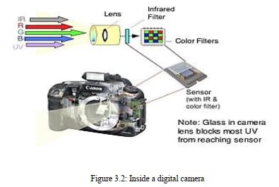
3.1.3 Techniques to Perform Image Acquisition

Picture Acquisition measure thoroughly relies upon the equipment framework which might have a sensor that is again an equipment gadget. A sensor changes over light into electrical charges. The sensor inside a camera estimates the reflected energy by the scene being imaged. The picture sensor utilized by most advanced cameras is a charge coupled gadget (CCD). A few cameras utilize corresponding metal oxide semiconductor (CMOS) innovation all things considered. Advanced cameras look a lot of like normal film cameras however they work in something else entirely. At the point when you press the button to snap a picture with a computerized camera, a gap opens at the front of the camera and light streams in from the perspective. Up until now, it's simply as old as film camera. Starting here on, be that as it may, everything is unique. There is no film in a computerized camera. All things considered, there is a piece of electronic hardware that catches the approaching light beams and transforms them into electrical signs. This light finder is one of two sorts, either a charge-coupled gadget (CCD) or a CMOS picture sensor. Assuming you've at any point checked out a TV screen close up, you will have seen that the image is comprised of millions of small shaded specks or squares called pixels. PC LCD PC screens likewise make up their pictures utilizing pixels, in spite of the fact that they are regularly excessively little to see. In a TV or PC screen, electronic gear turns this multitude of shaded pixels on and off rapidly. Light from the screen makes a trip out to your eyes and your mind is tricked into see a huge, moving picture. In an advanced camera, precisely the inverse occurs. Light from what you are capturing zooms into the camera focal point. This approaching "picture" hits the picture sensor chip, what splits it up into a large number of pixels. The sensor estimates the shading and brilliance of every pixel and stores it as a number. Your advanced photo is viably an immensely long series of numbers portraying the specific subtleties of every pixel it contains. When an image is put away in numeric structure, you can do a wide range of things with it. Attachment your computerized camera into your PC, and you can download the pictures you've taken and load them into programs like Photoshop to alter them or jazz them up. Or on the other hand you can transfer them onto sites, email them to companions, etc. This is conceivable in light of the fact that your photos are put away in computerized configuration and a wide range of other advanced contraptions—everything from MP3-playing iPods to cellphones and PCs to photograph printers—utilize computerized innovation as well. Computerized is a sort of language that every electronic contraption "talk" today. Taking an advanced photograph: taking a gander at the picture on the LCD screen. Digital cameras are significantly more advantageous than film cameras. You can right away perceive how the image will look from the LCD screen on the back. On the off chance that your image doesn't end up good overall, you can essentially erase it and attempt once more. You can't do that with a film camera. Advanced cameras mean photographic artists can be more imaginative and test. If you open up an advanced photo in a paint (picture altering) program, you can transform it in a wide range of ways. A program like this works by changing the numbers that address every pixel of the picture. In this way, on the off chance that you click on a control that makes the picture 20% more splendid, the program goes through every one of the numbers for every pixel thusly and expands them by 20%. In the event that you reflect a picture (flip it on a level plane), the program switches the arrangement of the numbers it stores so they run the other way. What you see on the screen is the picture changing as you alter or control it. Be that as it may, what you don't see is the paint program changing every one of the numbers behind the scenes. A portion of these picture altering methods are incorporated into more complex advanced cameras. You may have a camera that has an optical zoom and an advanced zoom. An optical zoom implies that the focal point moves in and out to make the approaching picture greater or more modest when it hits the CCD. A computerized zoom implies that the CPU inside the camera explodes the approaching picture without really moving the focal point. In this way, very much like drawing nearer to a TV set, the picture corrupts in quality. So, optical zooms make pictures greater and similarly as understood, however advanced zooms make pictures greater and more obscured. Imagine for a moment that you're a CCD or CMOS image sensing chip. Look out of a window and try to figure out how you would store details of the view you can see. First, you'd have to divide the image into a grid of squares. So, you'd need to draw an imaginary grid on top of the window. Next, you'd have to measure the color and brightness of each pixel in the grid. Finally, you'd have to write all these measurements down as numbers. If you measured the color and brightness for six million pixels and wrote both down both things as numbers, you'd end up with a string of millions of numbers—just to store one photograph! This is why high-quality digital images often make enormous files on your computer. Each one can be several megabytes (millions of characters) in size. To get around this, digital cameras, computers, and other digital gadgets use a technique called compression. Compression is a mathematical trick that involves squeezing digital photos so they can be stored with fewer numbers and less memory. One popular form of compression is called JPG (pronounced J-PEG, which stands for Joint Photographic Experts Group, after the scientists and mathematicians who thought up the idea). JPG is known as a "lossy" compression because, when photographs are squeezed this way, some information is lost and can never be restored. High-resolution JPGs use lots of memory space and look very clear; low resolution JPGs use much less space and look more blurred. You can find out more about compression in our article on MP3 players. Most digital cameras have settings that let you take pictures at higher or lower resolutions. If you select high-resolution, the camera can store fewer images on its memory card—but they are much better quality opt for low-resolution and you will get more images, but the quality won't be as good. Low-resolution images are stored with greater compression. Both CCD and CMOS picture sensors convert light into electrons. An improved-on approach to contemplate these sensors is to think about a 2-D cluster of thousands or millions of little sunbased cells. (For this situation the sensors are called photograph locales). When the sensor changes over the light into electrons, it peruses the worth (amassed charge) of every cell in the picture. A CCD transports the charge across the chip and peruses it at one corner of the exhibit. A simple to advanced converter (ADC) then, at that point transforms every pixel's worth into a computerized esteem by estimating the measure of charge at every photograph site and changing that estimation over to paired structure. CMOS gadgets utilize a few semiconductors at every pixel to enhance and move the charge utilizing more customary wires. CCD sensors make superior grade, low-commotion pictures. CMOS sensors are by and large more defenseless to commotion. CMOS sensors customarily devour little force comparable CMOS sensor. CCD sensors have been mass created for a more extended timeframe, so they are fuller grown. They will in general have more excellent pixels and a greater amount of them. The Image Acquisition is simply a Hardware Dependent Process, in which mirrored light energy from the item being imaged is changed over into electrons and spread over the interior sensor chip which resembles a 2-D exhibit of cells is cell is called photograph site and contain number of charges which is additionally changed over to advanced structure utilizing Analog to Digital Converter.

3.2 Image Preprocessing

Picture pre-preparing is the term for procedure on pictures at the most reduced degree of deliberation. These tasks don't build picture data content yet they decline it in case entropy is a data measure. The point of pre-handling is an improvement of the picture information that stifles undesired twists or upgrades some picture highlights important for additional preparing and investigation task. The point of pre-processing is to work on the nature of the picture with the goal that we can break down it in a superior manner. By preprocessing we can smother undesired twists and17 upgrade a few highlights which are essential for the specific application we are working for. Those elements may shift for various applications. For instance, assuming we are chipping away at an undertaking which can robotize Vehicle Identification, our principal center lies around the vehicle, its tone, the enrollment plate, and so forth, we don't zero in out and about or the sky or something which isn't required for this specific application. Envision, the PC can just say, "I'm ravenous!". You can take care of it with one or the other water or food. However, for the PC to work appropriately, you need to give it the fitting one which will make it work appropriately. Also, that is a similar explanation regarding the reason why we need to preprocess pictures prior to taking care of them to programs. We can straightforwardly give contributions to programs however those might yield an awful outcome which isn't precise. So, we are really assisting the PC with yielding great outcomes by giving it preprocessed information. There are 4 unique kinds of Image Pre-Processing methods and they are recorded below.

• Pixel brightness corrections

• Geometric Transformations

• Image Filtering and Segmentation

• Fourier transform and Image restauration

We will examine each type exhaustively.

3.2.1 Pixel Brightness Corrections

Splendor changes alter pixel brilliance and the change relies upon the properties of a pixel itself. In PBT, yield pixel's worth relies just upon the relating input pixel esteem. Instances of such administrators incorporate splendor and differentiation changes just as shading amendment and changes. Difference improvement is a significant region in picture preparing for both human and. CCDs, then again, utilize a cycle that devours bunches of force. It is broadly utilized for clinical picture preparing and as a pre-handling step in discourse acknowledgment, surface combination, and numerous other picture/videos preparing applications There are two kinds of Brightness changes and they are:

• Brightness corrections

• Gray scale transformation18

The most common Pixel brightness transforms operations are

• Gamma correction or Power Law Transform

• Sigmoid stretching

• Histogram equalization

Two ordinarily utilized point measures are multiplication and addition with a consistent. g(x)=αf(x)+β…………………………………….. 3.2 The boundaries α>0 and β are known as the addition and inclination boundaries and in some cases these boundaries are said to control contrast and brightness separately. For various upsides of alpha and beta, the picture brightness and contrast fluctuate.

3.2.2 Gamma Correction

Gamma correction is a non-direct change in accordance with individual pixel esteems. While in picture standardization we did straight procedure on individual pixels, like scalar augmentation and expansion/deduction, gamma adjustment completes a non-direct procedure on the source picture pixels, and can cause saturation of the picture being altered. Gamma correction is basically a power law change, aside from low luminance where it's direct in order to try not to have a boundless subordinate at luminance zero. This is the customary nonlinearity applied for encoding SDR pictures. For various upsides of alpha and beta, the picture brightness and contrast fluctuate. The type or "gamma", as determined in the business standard BT.709, has a worth of 0.45 however truth be told the direct piece of the lower some portion of the bend makes the last gamma revision work be more like a power law of type 0.5 for example a square root change: along these lines, gamma remedy follows the DeVries-Rose law of splendor discernment. Regardless we should take note of that camera producers regularly adjust marginally the gamma worth and it is a subject of exploration how to precisely assess gamma from a given picture. It's norm to encode the gamma remedied picture utilizing 8 pieces for each channel, regardless of the way that this piece profundity is scarcely enough for SDR pictures and creates banding in the lowlights. Consequently, 10 pieces are utilized in TV creation, despite the fact that transmission is finished with 8 pieces.

𝑜 = (255 𝐼 )𝛾 × 255…………………………………… 3.3

Here the connection between yield picture and gamma is nonlinear.

3.2.3 Histogram Equalization

A histogram of a picture is the graphical translation of the picture's pixel power esteems. It very well may be deciphered as the information structure that stores the frequencies of all the pixel power levels in the picture. It achieves this by successfully fanning out the most regular power esteems, for example loosening up the power scope of the picture. This technique as a rule expands the worldwide differentiation of pictures when its usable information is addressed by close difference esteems. This takes into account spaces of lower nearby differentiation to acquire a higher difference. A histogram of a picture is the graphical translation of the picture's pixel power esteems. It very well may be deciphered as the information structure that stores the frequencies of all the pixel power levels in the picture. Histogram equalization is a notable difference upgrade strategy because of its presentation on practically a wide range of pictures. Histogram equalization gives a modern strategy to adjusting the unique reach and difference of a picture by changing that picture with the end goal that its force histogram has the ideal shape. Not at all like difference extending, histogram displaying administrators might utilize non-direct and non-monotonic exchange capacities to plan between pixel force esteems in the info and yield pictures. P(n) = number of pixels with intensity n/all out the number of pixels.

3.3 Sigmoid Stretching

Sigmoid capacity is a persistent nonlinear actuation work. The name, sigmoid, is gotten from the way that the capacity is "S" formed. Analysts consider this capacity the logistic function. Sigmoid functions regularly show return esteem (y hub) in the reach 0 to 1. Another usually utilized reach is from one 1 to another. The contrast of any image is a very important characteristic by which the image can be judged as good or poor. In this paper, we introduce a simple approach for the process of image contrast enhancement using the sigmoid function in spatial domain. To achieve this simple contrast enhancement, a novel mask based on using the input value together with the sigmoid function formula in an equation that will be used as contrast enhancer.

𝑓(𝑥) = 1/1+𝑒−𝑡𝑥…………………………………… 3.4

𝑔(𝑥, 𝑦) = 1/1+𝑒(𝑐∗(𝑡ℎ−𝑓𝑠(𝑥,𝑦)))…………………………..… 3.5

g (x,y) is Enhanced pixel esteem

c is Contrast factor

th is Threshold esteem

fs(x,y) is original picture

By changing the difference factor 'c' and limit esteem it is feasible to tailor the measure of easing up and obscuring to control the general differentiation improvement.

3.4 Geometric Transformations

As perceived by the name, it implies changing the calculation of a picture. A bunch of picture changes where the calculation of picture is changed without modifying its genuine pixel esteems are ordinarily alluded to as "Mathematical" change. As a general rule, you can apply different procedure on it, however, the real pixel esteems will stay unaltered. In these changes, pixel esteems are not changed, the places of pixel esteems are changed. The main inquiry is, the thing that is the utilization of these mathematical changes, in actuality. So here we will give a few models where you can identify with the theme. For instance, some individual is clicking photos of similar spot at various times and year to envision the changes. Each time he taps the image, it's excessive that he taps the image at precisely the same point. So, for better perception, he can adjust every one of the pictures at a similar point utilizing mathematical change.

3.5 Image Filtering and Segmentation

Picture filtering includes the use of window activities that perform valuable capacities, for example, commotion expulsion and picture upgrade. This section is concerned especially with what can be accomplished with very essential channels, like mean, middle, and mode channels. Strangely, these channels effect sly affect the states of articles; truth be told, the investigation of shape occurred throughout a significant stretch of time and brought about a profoundly variegated arrangement of calculations and techniques, during which the all-encompassing formalism of numerical morphology was set up. This part directs a natural way between the numerous numerical hypotheses, showing how they lead to for all intents and purposes valuable procedures. The objective of utilizing channels is to adjust or improve picture properties or potentially to separate significant data from the photos like edges, corners, and masses. A channel is characterized by a portion, which is a little cluster applied to every pixel and its neighbors inside a picture. Some of the basic filtering techniques are

1. Low Pass Filtering (Smoothing): A low pass channel is a reason for most smoothing techniques. A picture is smoothed by diminishing the dissimilarity between pixel esteems by averaging close by pixels.

2. High pass filters (Edge Detection, Sharpening): High-pass channel can be utilized to cause a picture to seem more honed. These channels underline fine subtleties in the picture – something contrary to the low-pass channel. High-pass separating works similarly as low-pass sifting; it simply utilizes an alternate convolution bit.

3. Directional Filtering: Directional channel is an edge finder that can be utilized to register the primary subordinates of a picture. The principal subordinates (or slants) are most clear when a huge change happens between contiguous pixel esteems. Directional channels can be intended for any bearing inside a given space.

4. Laplacian Filtering: The laplacian channel is an edge finder used to register the second subordinates of a picture, estimating the rate at which the principal subsidiaries change.

   3.5.1 Image Segmentation

   Image segmentation is a usually utilized method in advanced picture preparing and investigation to parcel a picture into different parts or areas, regularly dependent on the attributes of the pixels in the picture. Picture segmentation could include isolating frontal area from foundation, or bunching locales of pixels dependent on likenesses fit as a fiddle. Image Segmentation chiefly utilized in

• Face detection

• Medical imaging

• Machine vision

• Autonomous Driving

A computerized picture is comprised of different parts that should be "investigated", how about we utilize that word for straightforwardness purpose and the "examination" performed on such parts can uncover a great deal of concealed data from them. This data can assist us with tending to a plenty of business issues – which is one of the many ultimate objectives that are connected with picture handling. Picture Segmentation is the cycle by which a computerized picture is apportioned into different subgroups (of pixels) called Image Objects, which can lessen the intricacy of the picture, and hence breaking down the picture becomes less complex. The idea of apportioning, separating, getting, and afterward naming and later utilizing that data to prepare different ML models have for sure tended to various business issues. In this part, how about we attempt to get what issues are addressed by Image Segmentation. A facial acknowledgment framework executes picture division, recognizing a representative and empowering them to stamp their participation consequently. Division in Image Processing is being utilized in the clinical business for productive and quicker analysis, recognizing sicknesses, growths, and cell and tissue designs from different clinical symbolism created from radiography, MRI, endoscopy, thermography, ultrasonography, and so on .Satellite pictures are handled to distinguish different examples, objects, topographical forms, soil data and so on, which can be subsequently utilized for horticulture, mining, geodetecting, and so on Picture division has a huge application region in mechanical technology,as RPA, self-driving vehicles, and so on Security pictures can be handled to recognize hurtful articles, dangers, individuals and occurrences. Picture division executions in python, MATLAB and different languages are broadly utilized for the interaction. An extremely intriguing case we coincidentally found was a show about a specific food handling processing plant on the Television, where tomatoes on a quick transport line were being examined by a PC. It was taking fast pictures from a reasonably positioned camera and it was passing guidelines to an attractions robot which was get spoiled ones, unripe ones, fundamentally, harmed tomatoes and permitting the great ones to pass on. This is a fundamental, however an essential and critical utilization of Image Classification, where the calculation had the option to catch just the necessary parts from a picture, and those pixels were later being named the general mishmash by the framework. A fairly basic looking framework was having a titanic effect on that business – killing human exertion, human blunder and expanding effectiveness. We utilize different picture division calculations to part and gathering a specific arrangement of pixels together from the picture. Thusly, we are really allotting marks to pixels and the pixels with a similar name fall under a class where they have a few or the other thing normal in them. Utilizing these marks, we can indicate limits, define boundaries, and separate the most required articles in a picture from the remainder of the not-really significant ones. In the underneath model, from a fundamental picture on the left, we attempt to get the significant parts, for example seat, table and so on and consequently every one of the seats are shaded consistently. In the following tab, we have identified occurrences, which talk about individual items, and henceforth the every one of the seats have various shadings. There are two types of image segmentation approaches:

• Non-contextual Thresholding

• Contextual Thresholding

Non-contextual Thresholding: Thresholding is the least complex non-contextual segmentation procedure. With a solitary threshold, it changes a greyscale or shading picture into a binary picture considered as a binary region map. The binary region map contains two potentially disjoint areas, one of them containing pixels with input information esteems less25 than an edge and another identifying with the information esteems that are at or over the limit. The following are the kinds of thresholding methods.

• Simple thresholding

• Adaptive thresholding

• Color thresholding

Contextual Segmentation: non-contextual thresholding bunches pixels with no record of their overall areas in the picture plane. Contextual division can be more fruitful in isolating individual articles since it represents closeness of pixels that have a place with a singular item. Two essential ways to deal with logical division depend on signal brokenness or likeness. Brokenness based strategies endeavor to discover total limits encasing generally uniform areas accepting sudden sign changes across every limit. Closeness based procedures endeavor to straightforwardly make these uniform districts by gathering associated pixels that fulfill certain similitude measures. Both the methodologies reflect one another, as in a total limit parts one area into two. The underneath are the kinds of Contextual division.

• Pixel connectivity

• Region similarity

• Region growing

• Split-and-merge segmentation

3.6 Fourier Transform

The Fourier Transform is a significant picture preparing device which is utilized to break down a picture into its sine and cosine parts. The yield of the change addresses the picture in the Fourier or recurrence space, while the info picture is the spatial area same. In the Fourier space picture, each point addresses a specific recurrence contained in the spatial area picture. The Fourier Transform is utilized in a wide scope of utilizations, for example, picture investigation, picture separating, picture reproduction and picture pressure. The discrete Fourier change is the inspected Fourier Transform and hence doesn't contain all frequencies framing a picture, however just a bunch of tests which is sufficiently enormous to completely portray the spatial space picture. For a square picture of size N×N, the two-dimensional DFT is given by: Inverse Fourier Transform is given by The Fourier transform disintegrates a picture into its sine and cosine parts. Set forth plainly, sine and cosine are waves beginning at any rate and most extreme separately. In reality, we can't figure out if a wave that we notice began at a most extreme or least point, and hence we can't actually recognize the two. Consequently, sine and cosine are essentially alluded to as sinusoids. While applying the FT to a picture, we change it from its spatial area into a "recurrence area", which generally is the picture addressed as far as its variety in shading and splendor over the long run (all things considered, not time, however space. That is, over various pixels). The Fourier change of a picture separates the picture work (the undulating scene) into an amount of constituent sine waves. Similarly concerning a sound wave, the Fourier change is plotted against recurrence. In any case, in contrast to that circumstance, the recurrence space has two aspects, for the frequencies h and k of the waves in the x and y aspects. So, it is plotted not as a progression of spikes, but rather as a picture with (generally) similar aspects in pixels as the first picture. Every pixel in the Fourier change has a facilitate (h,k) addressing the commitment of the sine wave with x-recurrence h, and y-recurrence k in the Fourier change. The middle point addresses the (0,0) wave – a level plane without any waves – and its power (its brilliance in shading in the dim scale) is the normal worth of the pixels in the picture. The focuses to the left and right of the middle, address the sine waves that change along the x-hub, (k=0). The splendor of these focuses addresses the force of the sine wave with that recurrence in the Fourier change (the power is the plentifulness of the sine wave, squared). Those in an upward direction above and beneath the middle point address those sine waves that shift in y,27 however stay steady in x (h=0). Furthermore, different focuses in the Fourier change address the commitments of the askew waves. The Fourier changes of straightforward blends of waves have a couple of splendid spots. In any case, for more perplexing pictures, for example, advanced photographs, there are numerous many brilliant spots in its Fourier change, as it takes many waves to communicate the picture. In the Fourier change of numerous advanced photographs, we'd ordinarily take, there is regularly a solid force along the x and y hub of the Fourier change, showing that the sine waves that just shift along these tomahawks have a major influence in the last picture. This is on the grounds that there are numerous levels or vertical highlights and balances in our general surroundings – dividers, table tops, even bodies are even around the upward tomahawks. You can see this by turning a picture a bit (say by 45%). Then, at that point, its Fourier change will have a solid force along a couple of opposite lines that are turned by a similar sum. Fourier changes are inconceivably valuable devices for the investigation and control of sounds and pictures. Specifically for pictures, it's the numerical apparatus behind picture pressure, (for example, the JPEG design), sifting pictures and lessening obscuring and commotion.

3.7 Input to Pre- trained Model

A model that has autonomously taken in prescient connections from preparing information, regularly utilizing AI is called pre trained model. A pre-trained model is a saved network that was previously trained on a large dataset, typically on a large-scale image-classification task. You either use the pretrained model as is or use transfer learning to customize this model to a given task. The intuition behind transfer learning for image classification is that if a model is trained on a large and general enough dataset, this model will effectively serve as a generic model of the visual world. You can then take advantage of these learned feature maps without having to start from scratch by training a large model on a large dataset. The human mind can28 undoubtedly perceive and recognize the articles in a picture. For example, given the picture of a feline and canine, inside nanoseconds, we recognize the two and my mind sees this distinction. On the off chance that a machine emulates this conduct, it is as near Artificial Intelligence we can get. Therefore, the field of Computer Vision intends to copy the human vision framework – and there have been various achievements that have broken the boundaries in such manner. In addition, these days machines can undoubtedly recognize various pictures, distinguish items and faces, and even create pictures of individuals who don't exist! This very capacity of a machine to recognize objects prompts more roads of examination – like recognizing individuals. The fast advancements in Computer Vision, and likewise – picture characterization has been additionally sped up by the coming of Transfer Learning. To lay it out plainly, Transfer learning permits us to utilize a previous model, prepared on a gigantic dataset, for our own undertakings. Thus, decreasing the expense of preparing new profound learning models and since the datasets have been checked, we can be guaranteed of the quality. In Image Classification, there are some extremely famous datasets that are utilized across exploration, industry, and hackathons. A pre-prepared model addresses a model that was prepared for a specific assignment on the ImageNet informational collection. This entire cycle is called Transfer Learning and it's in reality a bit something other than bringing a model into your work space. Our model is named Faster RCNN. It is a Combination of RPN (Region proposed network) and Fast RCNN. It contains 02 main layers:

1. Classifier

2. Regressor

There are a few considerable advantages that urges me to pick Faster RCNN models: • super easy to join.

• achieve strong (same or far better) model execution rapidly.

• there's not as much marked information required.

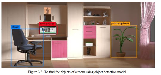
3.8 Object Detection

It is a computer vision strategy for finding cases of items in pictures or recordings. Item discovery calculations commonly influence AI or profound figuring out how to create significant outcomes. At the point when people take a gander at pictures or video, we can perceive and find objects of interest inside a question of minutes. The objective of article identification is to repeat this knowledge utilizing a PC. Object recognition is an overall term to portray an assortment of related PC vision undertakings that include distinguishing objects in computerized photos. Image classification includes anticipating the class of one article in a picture. Item limitation alludes to distinguishing the area of at least one articles in a picture and drawing flourishing box around their degree. Object detection joins these two undertakings and restricts and orders at least one articles in a picture.

All things considered; we can recognize these PC vision tasks:

Picture Classification: Predict the sort or class of an item in a picture.

Input: A picture with a solitary article, like a photo.

Output: A class mark (for example at least one numbers that are planned to class names).

Article Localization: Locate the presence of items in a picture and show their area with a jumping box. Input: A picture with at least one articles, like a photo.

Output: at least one bouncing boxes (for example characterized by a, width, and stature).

Article Detection: Locate the presence of items with a jumping box and types or classes of the found articles in a picture.

Input: A picture with at least one articles, like a photo.

Output: at least one jumping boxes (for example characterized by a, width, and tallness), and a class mark for each bouncing box.

Article identification: Algorithms produce a rundown of item classifications present in the picture alongside a hub adjusted jumping box demonstrating the position and size of each occasion of each item class.

We can see that "Single-object localization" is a less complex rendition of the more extensively characterized "Item Localization," obliging the localization tasks to objects of one sort inside a picture, which we might accept that is an easier task. Picture grouping: Algorithms produce a rundown of item classifications present in the picture. Single-object localization: Algorithms produce a rundown of item classifications present in the picture, alongside a pivot adjusted jumping box showing the position and size of one occasion of each article classification. One further augmentation to this breakdown of PC vision errands is object division, likewise called "object occasion division" or "semantic division," where occurrences of perceived items are shown by featuring the particular pixels of the article rather than a coarse jumping box. A large portion of the new advancements in picture acknowledgment issues have come as a feature of cooperation in the ILSVRC assignments. This is a yearly scholarly rivalry with a different test for every one of these three issue types, with the goal of cultivating autonomous and separate upgrades at each level that can be utilized all the more extensively. For instance, see the rundown of the three relating task types underneath taken from the 2015 ILSVRC survey paper: Object detection is a vital innovation behind cutting edge driver help frameworks that empower vehicles to distinguish driving paths or perform walker location to further develop street security.31 Item recognition is likewise valuable in applications like video reconnaissance or picture recovery frameworks. We can browse two critical ways to deal with begin with object detection:

• Make and train a custom detector. To prepare a custom object detector without any preparation, you need to plan an organization engineering to become familiar with the components for the objects of interest. You additionally need to gather an extremely enormous arrangement of marked information to prepare the CNN. The consequences of a custom object detector can be astounding. All things considered, you need to physically set up the layers and loads in the CNN, which requires a great deal of time and preparing information.

• Utilize a pretrained object finder. Many item recognition work processes utilizing profound learning influence move learning, a methodology that empowers you to begin with a pretrained organization and afterward adjust it for your application. This technique can give quicker outcomes on the grounds that the item indicators have as of now been prepared on thousands, or even millions, of pictures.

As we mentioned before we used pretrained model for my work.

3.9 Dataset

A dataset in PC vision is a curated set of advanced photos that designers use to test, prepare and assess the exhibition of their calculations. The calculation is said to gain from the models contained in the dataset. What realizing implies in this setting has been depicted by Alan Turing (1950): "it is ideal to give the machine the most amazing receptors available anywhere, and afterward encourage it to comprehend and communicate in English. This interaction could follow the typical instructing of a youngster. Things would be brought up and named, and so forth" A dataset in PC vision thusly gathers an assortment of pictures that are named and utilized as references for objects on the planet, to 'call attention to things' and name them. PC vision datasets rely upon the accessibility of huge volumes of photos. Every class of ImageNet allegedly contains at least 1000 pictures and classifications incorporate an immense assortment of points from plants and geographical arrangements to people and creatures. Simultaneously, the measure of comment work engaged with the creation of datasets is considerably more amazing than the measure of photographs it contains Crafted by physically cross-referring to and naming the photographs is the thing that makes datasets like ImageNet so unique. Truth be told, there has been once in a while in the set of experiences such countless individuals paid to take a gander at pictures and report what they find in them (Krishna et al, 2016). The robotization of vision has not diminished however expanded the quantity of eyeballs taking a gander at pictures, of hands composing depictions, of taggers and annotators. However, what has changed is the setting wherein the movement of seeing is occurring, how retinas are snared in intensely specialized conditions and how vision is driven by an unprecedented speed. The MS COCO dataset is a huge scope object discovery, division, and inscribing dataset distributed by Microsoft. AI and Computer Vision designs famously utilize the COCO dataset for different PC vision projects. Understanding visual scenes is an essential objective of PC vision; it includes perceiving what articles are available, limiting the items in 2D and 3D, deciding the items ascribes, and describing the connection between objects. Along these lines, calculations for object discovery and article order can be prepared utilizing the dataset. COCO represents Common Objects in Context, as the picture dataset was made determined to propel picture acknowledgment. The COCO dataset contains testing, top notch visual datasets for PC vision, generally cutting-edge neural organizations. For instance, COCO is regularly used to benchmark calculations to think about the presentation of continuous article recognition. The configuration of the COCO dataset is naturally deciphered by cutting edge neural organization libraries. The huge dataset includes commented on photographs of regular scenes of normal articles in their normal setting. Those articles are marked utilizing pre-characterized classes, for example, "seat" or "banana". The most common way of marking, additionally named picture comment and is an extremely well-known procedure in PC vision. While other item acknowledgment datasets have zeroed in on

• picture characterization

• object bouncing box confinement

• semantic pixel-level division – the MS coco dataset centers around33

For some classes of articles, there are notable perspectives accessible. For instance, when playing out an electronic picture look for a particular item class (for instance, "seat"), the highest-level models show up in profile, un-deterred, and close to the focal point of an extremely coordinated photograph.

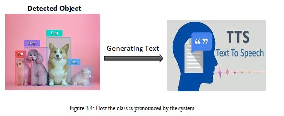
3.10 Image to Text Then Text to Voice

This method defines that subsequent to characterizing the item it will compose the class name. Our capacity plays out this activity to extricate the class of the item. Then, at that point the class name will be articulated by the PC through TTS. In this chapter, we discussed about the methodology my project. To build up our project we follow some steps. Step by step we established my project. We have COCO dataset, developed by Microsoft, and implement it.

Chapter 4

Algorithm

This section provides brief algorithm information from the disciplines contributing to this thesis: Finding an effective pathway for blind people using image classification and voice Command. First presented details of Convolution Neural Network. Next introduced are topics related to Convolution Neural Network: Convolution layer, Stride, Padding Non-Linearity (ReLU), Pooling Layer, Fully Connected Layer. Finally covered with a brief description of Faster RCNN.

4.1 Convolutional Neural Network (CNN)

In neural networks, Convolutional neural network is one of the core classes to do images recognition, images classifications. Object’s detections, recognition faces etc., are some of the parts where CNNs are broadly used. The convolutional neural network, or CNN for short, is a particular sort of neural organization model intended for working with two-dimensional picture information, in spite of the fact that they can be utilized with one-dimensional and three-dimensional information. Key to the convolutional neural network is the convolutional layer that gives the organization its name. This layer plays out an activity called a "convolution". With regards to a convolutional neural network, a convolution is a straight activity that includes the duplication of a bunch of loads with the info, similar as a customary neural organization. Considering that the method was intended for two-dimensional info, the increase is performed between a variety of information and a two-dimensional exhibit of loads, called a channel or a bit. The channel is more modest than the info information and the kind of increase applied between a channel measured fix of the info and the channel is a dab item. A dab item is the component shrewd increase between the channel measured fix of the info and channel, which is then added, continually bringing about a solitary worth. Since it brings about a solitary worth, the activity is frequently alluded to as the "scalar item". Utilizing a channel more modest than the info is deliberate as it permits a similar channel (set of loads) to be increased by the information exhibit on various occasions at various focuses on the info. In particular, the channel is applied deliberately to each covering part or channel measured fix of the information, passed on to right, start to finish. This methodical use of a similar channel across a picture is an influential thought. In the event that the channel is intended to identify a particular sort of component in the info, then, at that point, the use of that channel efficiently across the whole information picture permits the channel a chance to find that include anyplace in the picture. This capacity is regularly alluded to as interpretation in change, for example the overall interest in whether the component is available as opposed to where it was available. 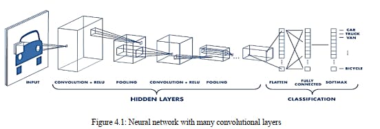Convolutional neural network image classifications have an input image, process it and classify it under specific groups (E.g., Dog, Cat, Tiger, Lion). Processers accepts an info picture as exhibit of pixels and it relies upon the picture goal. In view of the picture goal, it will get h × w × d (h = Height, w = Width, d = Dimension). E.g., A picture of 6 × 6 × 3 exhibits of network of RGB (3 alludes to RGB esteems) and a picture of 4 × 4 × 1 cluster of lattices of grayscale picture. Theoretically, deep learning Convolutional neural network models to train and trial, each input image will pass it through a series of convolution layers with filters (Kernels), Pooling, fully connected layers (FC) and apply Soft-max function to categorize an object with probabilistic values between 0 and 1. The below figure is a complete flow of Convolutional neural network to process an input image and categorizes the objects based on principles.

4.1.1 Convolution Layer

Convolution is the main layer to separate components from an information picture. Convolution protects the connection between pixels by learning picture highlights utilizing little squares of info information. It is a numerical activity that takes two sources of info, for example, picture grid and a channel or piece.

• An image matrix(volume) of dimension (h×w×d)

• A filter (𝑓ℎ × 𝑓𝑤 × 𝑑)

• Outputs a volume dimension (ℎ − 𝑓ℎ + 1) × (𝑤 − 𝑓ℎ + 1) × 1………………………. 4.1 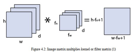Let a 5 × 5 whose image pixel values are 0, 1 and filter matrix 3 × 3 as given in below 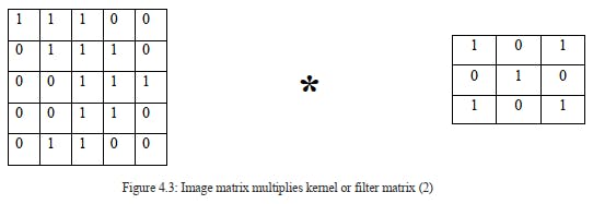Then, at that point the convolution of 5 × 5 picture grid duplicates with 3 × 3 channel network which is classified "Feature Map". Convolution of a picture with various channels can perform tasks, for example, edge location, obscure and hone by applying channels. Convolutional layers are the major building blocks used in convolutional neural networks. A convolution is the straightforward use of a channel to an information that outcomes in an enactment. Rehashed use of a similar channel to an information brings about a guide of initiations called an element map, demonstrating the areas and strength of a distinguished element in an information, like a picture. The development of convolutional neural organizations is the capacity to consequently get familiar with an enormous number of channels in equal explicit to a preparation dataset under the requirements of a particular prescient demonstrating issue, for example, picture arrangement. The outcome is exceptionally explicit components that can be identified anyplace on input pictures.

4.1.2 Stride

Stride is the quantity of pixels shifts over the information grid. At the point when the stride is 1 then we move the channels to 1 pixel at a time. At the point when the stride is 2 then we move the channels to 2 pixels all at once, etc. The underneath figure shows convolution would work with a stride of 2. 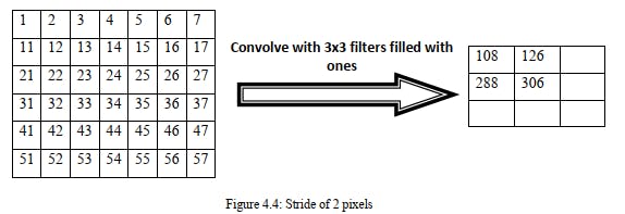Stride is a part of convolutional neural organizations, or neural organizations tuned for the pressure of pictures and video information. Step is a boundary of the neural organization's channel that changes the measure of development over the picture or video. For instance, if a neural organization's step is set to 1, the channel will move one pixel, or unit, at a time. The size of the channel influences the encoded yield volume, so step is frequently set to an entire whole number, rather than a small portion or decimal. Imagine a convolutional neural organization is taking a picture and examining the substance. In the event that the channel size is 3x3 pixels, the contained nine pixels will be changed over down to 1 pixel in the yield layer. Normally, as the step, or development, is expanded, the subsequent yield will be more modest. Step is a boundary that works related to cushioning, the component that adds clear, or void pixels to the edge of the picture to take into consideration a limited decrease of size in the yield layer. Generally, it is a method of expanding the size of a picture, to neutralize the way that step diminishes the size. Cushioning and step are the central boundaries of any convolutional neural organization. Stride is a significant idea in advanced picture handling. It permits playing out a few activities with a picture in an extremely quick way (in steady time) by straightforward change of picture metadata.

4.1.3 Padding

Padding is a term pertinent to convolutional neural organizations as it alludes to the measure of pixels added to a picture when it is being handled by the part of a CNN. For instance, assuming the cushioning in a CNN is set to nothing, every pixel esteem that is added will be of worth zero. Assuming, in any case, the zero cushioning is set to one, there will be a one-pixel line added to the picture with a pixel worth of nothing. Now and then channel doesn't fit impeccably with the information picture. We have two choices:

• Pad the image with zeros so it fits

• Drop the piece of the picture where the channel didn't fit. This is called legitimate padding which keeps just substantial piece of the picture.

As we recently talked about, the convolutional layers lessen the size of the yield. So, in situations where we need to expand the size of the yield and save the data introduced in the corners, we can utilize cushioning layers where cushioning helps by including additional lines and segments the external element of the pictures. So, the size of info information will stay like the yield information. Cushioning essentially broadens the space of a picture wherein a convolutional neural organization process. The part/channel which gets across the picture examines every pixel and39 converts the picture into a more modest picture. To work the portion with handling in the picture, cushioning is added to the external casing of the picture to consider more space for the channel to cover in the picture. Adding cushioning to a picture handled by a CNN takes into account a more precise examination of pictures. we have perceived how we can manage the issue of the straightforward convolutional layer by utilizing diverse cushioning. We have perceived how these cushioning techniques are not quite the same as one another. Where we can utilize something very similar and substantial cushioning with two-dimensional convolutional layers and causal cushioning with one-dimensional convolutional layers. At times, all the same, you really want to apply channels of a proper size, yet you would rather not lose width or potentially tallness aspects in your component maps. For instance, this is the situation when you're preparing an auto encoder. You really want the yield pictures to be of a similar size as the info, yet need an enactment work like for example Sigmoid to produce them. If you would do as such with a Convolution layer, this would become tricky, as you'd decrease the size of your element maps – and consequently would deliver yields inconsistent in size to your bits of feedbacks. That is not what we need when we make an auto encoder. We need the first yield and the first yield as it were Cushioning assists you with taking care of this issue. Applying it successfully adds "space" around your feedback information or your element map – or, all the more definitively, "additional lines and segments" Padding works by expanding the space of which a convolutional neural organization processes a picture. The bit is the neural organizations channel which gets across the picture, checking every pixel and changing over the information into a more modest, or now and again bigger, design. To help the part with handling the picture, padding is added to the edge of the picture to take into consideration more space for the portion to cover the picture. Adding padding to a picture handled by a CNN takes into account more exact examination of pictures.

4.2 Non-Linearity (ReLU)

ReLU represents Rectified Linear Unit for a non-direct activity. This yield is f(x)=max (0, x). Why ReLU is significant: ReLU's motivation is to present non-linearity in our ConvNet. Since, this present reality information would need our ConvNet to learn would be non-negative direct qualities. There are other non-straight capacities, for example, tanh or sigmoid that can likewise be utilized rather than ReLU. The majority of the information researchers use ReLU since execution savvy ReLU is superior to the next two. To utilize stochastic gradient plummet with backpropagation of mistakes to prepare profound neural organizations, an actuation work is required that looks and behaves like a straight capacity, however is, truth be told, a nonlinear capacity permitting complex connections in the information to be learned. The capacity should likewise give greater affectability to the initiation aggregate information and keep away from simple immersion. The arrangement had been skipping around in the field for quite a while, despite the fact that was not featured until papers in 2009 and 2011 focused a light on it. The arrangement is to utilize the corrected direct initiation capacity, or ReLU for short. A hub or unit that executes this enactment work is alluded to as a corrected direct initiation unit, or ReLU for short. Regularly, networks that utilization the rectifier work for the secret layers are alluded to as redressed networks. Reception of ReLU may effectively be viewed as one of a handful of the achievements in the profound learning upset, for example the strategies that currently license the normal improvement of exceptionally profound neural organizations. The corrected straight enactment work is a straightforward computation that profits the worth gave as information straightforwardly, or the worth 0.0 if the information is 0.0 or less.

4.3 Pooling Layer

Pooling layers area would decrease the quality of boundaries when the pictures are excessively enormous. Spatial pooling likewise called subsampling or down examining which diminishes the dimensionality of each guide however holds significant data. Spatial pooling can be of various sorts:

• Max Pooling

• Average Pooling

• Sum Pooling

Max pooling takes the biggest component from the redressed include map. Taking the biggest component could likewise take the normal pooling. Amount of all components in the element map call as sum pooling. 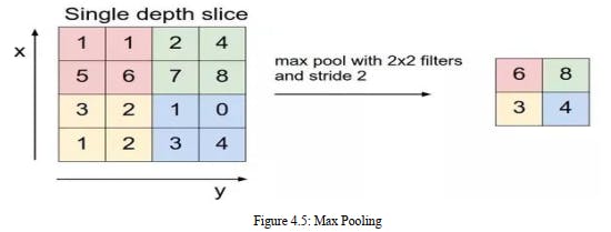Pooling basically helps in separating sharp and smooth elements. It is additionally done to lessen difference and calculations. Max-pooling helps in extricating low-level highlights like edges, focuses, and so on While Avg-pooling goes for smooth highlights. Assuming time requirement isn't an issue, one can skirt the pooling layer and utilize a convolutional layer to do likewise. Max pooling picks the discrete most extreme on the pixel framework, which commonly isn't the genuine greatest. In the event that your limit of your element turns out to be in 4 pixels, you will pass on a more fragile worth ahead. Average pooling accepts a solitary mode with a solitary centroid, if your dispersion has more than one mode or you have exceptions, your normal pooling will not be exact. Average Pooling is a pooling activity that computes the normal incentive for patches of an element map, and uses it to make a down sampled (pooled) highlight map. It is normally utilized after a convolutional layer. It adds a limited quantity of interpretation in variance - which means deciphering the picture just barely doesn't altogether influence the upsides of most pooled yields. It separates includes more flawlessly than Max Pooling, though max pooling extricates more articulated components like edges. Convolutional Neural Networks work effectively in managing high dimensional information. Confining the quantity of loads just to bits loads makes learning simpler because of invariance properties of pictures or sound. Yet, if you cautiously check out what's happening you might see that the after first convolutional layer the component of your information may seriously increment if you don't do the stunts like pooling. Max pooling diminishes the component of your information essentially by taking just the most extreme contribution from a decent area of your convolutional layer. Total pooling works in a similar way - by taking the number of contributions rather than its most extreme. The reasonable distinction between these methodologies lies in the kind of invariance which they can get. Max pooling is delicate to presence of some example in pooled district. Total pooling (which is relative to Mean pooling) measures the mean worth of presence of an example in a given area. The subregions for Sum pooling/Mean pooling are set precisely as old as Max pooling however rather than utilizing max work you use aggregate/mean.

4.3.1 Fully Connected Layer

CNN is a kind of profound learning model for handling information that has a lattice design, like pictures, which is motivated by the association of creature visual cortex and intended to naturally and deceptively learn spatial chains of command of highlights, from low-to significant level examples. CNN is a numerical develop that is normally made out of three sorts of layers (or building blocks): convolution, pooling, and completely associated layers. The initial two, convolution and pooling layers, perform highlight extraction, though the third, a completely associated layer, maps the removed elements into conclusive yield, like order. A convolution layer assumes a vital part in CNN, which is made out of a heap of numerical activities, like convolution, a specific sort of straight activity. In computerized pictures, pixel esteems are put away in a two-dimensional (2D) network, i.e., a variety of numbers and a little matrix of boundaries called bit, an optimization element extractor, is applied at each picture position, which makes CNN's exceptionally effective for picture handling, since an element might happen any place in the picture. The layer we call as fully connected layers, we leveled my framework into vector and feed it into a completely associated layer like a neural organization. 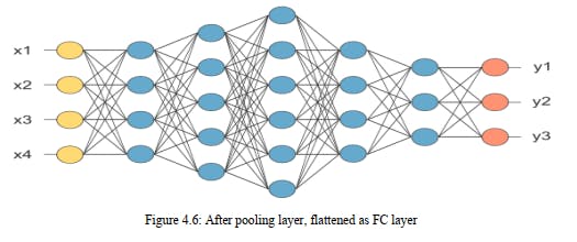As one layer takes care of its yield into the following layer, extricated elements can progressively and dynamically turn out to be more intricate. The method involved with improving boundaries, for example, pieces is called preparing, which is performed in order to limit the contrast among yields and ground truth names through an advancement calculation called back propagation and slope plummet, among others. In the above chart, the feature map grid will be changed over as vector (x1, x2, x3, …). With the completely associated layers, we consolidated these components together to make a model. At last, we have an initiation capacity like soft max or sigmoid to order the yields as feline, canine, vehicle, truck and so forth, Convolutional neural network (CNNs) addresses a fascinating technique for versatile picture handling, and structure a connection between broad feed-forward neural organizations and versatile channels. Two dimensional CNNs are shaped by at least one layers of two-dimensional channels, with conceivable non-direct actuation capacities and additionally down-inspecting. CNNs have key properties of interpretation invariance and spatially nearby associations (responsive fields). We present a portrayal of the convolutional network engineering, and an application to commonsense picture handling on a versatile robot. A CNN is utilized to distinguish and describe breaks on an independent sewer assessment robot. The channel sizes utilized in all cases were 4x4, with non-straight actuations between each layer. The quantity of component maps utilized in the three secret layers was, from contribution to yield, 4, 4, 4. The organization was prepared utilizing a dataset of 48x48 sub-areas drawn from 30 actually picture 320x240 pixel outlines examined from a pre-recorded sewer pipe review video. 15 casings were utilized for preparing and 15 for approval of organization execution. 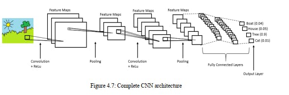The outcomes support the idea that information based versatile picture handling strategies, for example, CNNs are helpful for picture handling, or different applications where the information exhibits are huge, and spatially/transiently conveyed. Further refinements of the CNN engineering, like the execution of divisible channels, or augmentations to three-dimensional (i.e., Video) handling, are recommended.

4.4 Faster RCNN

A faster RCNN object recognition network is made out of an element extraction network, is ordinarily a pretrained CNN, like what we had utilized for its archetype. This is then trailed by two subnetworks which are teachable. The first is a Region Proposal Network (RPN), which is, as its name recommends, used to create object recommendations and the second is utilized to foresee the genuine class of the article. So, the essential differentiator for Faster R-CNN is the RPN which is embedded after the last convolutional layer. This is prepared to create district proposition straightforwardly without the requirement for any outside instrument like Selective Search. After this we use ROI pooling and an upstream classifier and bounding box regressor like Fast R-CNN.

4.4.1 Architecture and Design

Faster R-CNN is an expansion of Fast R-CNN. As its name recommends, Faster R-CNN is quicker than Fast R-CNN because of the area proposition organization (RPN). The fundamental commitments in this model are: Proposing locale proposition organization (RPN) which is a completely convolutional network that creates recommendations with different scales and perspective proportions. The RPN executes the wording of neural organization with thoughtfulness regarding tell the item discovery (Fast R-CNN) where to look. 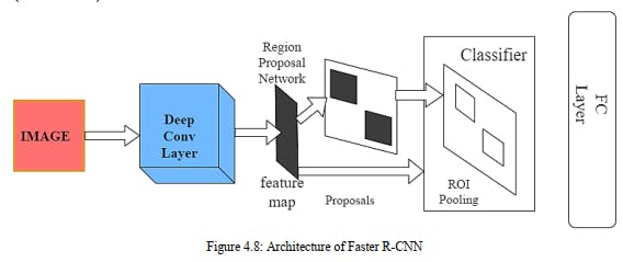Maybe than utilizing pyramids of pictures (for example numerous occasions of the picture yet at various scales) or pyramids of channels (for example various channels with various sizes), this paper presented the idea of anchor boxes. An anchor box is a reference box of a particular scale and viewpoint proportion. With different reference anchor boxes, then, at that point, numerous scales and perspective proportions exist for the single area. This can be considered as a pyramid of reference anchor boxes. Every area is then planned to each reference anchor box, and in this way distinguishing objects at various scales and angle proportions. The convolutional calculations are shared across the RPN and the Fast R-CNN. This lessens the computational time. The engineering of Faster R-CNN is displayed in the following figure. It comprises of 2 modules:

• RPN: For producing area proposition.

• Fast R-CNN: For recognizing objects in the proposed areas.

The RPN module is liable for creating locale proposition. It applies the idea of consideration in neural organizations, so it directs the Fast R-CNN identification module to where to search for objects in the picture.

The Faster R-CNN works as follows:

The RPN creates area recommendations. For all district proposition in the picture, a fixed-length include vector is removed from every area utilizing the ROI Pooling layer. The extricated include vectors are then characterized utilizing the Fast R-CNN. The class scores of the identified items notwithstanding their jumping boxes are returned.

• Regional Proposal Network (RPN): The objective of RPN is to yield a bunch of recommendations, every one of which has a score of its likelihood of being an item and furthermore the class/name of the article. RPN can take any estimated contribution to accomplish this undertaking. These propositions are additionally refined by taking care of to 2 kin completely associated layers-one for bouncing box relapse and the other for box characterization i.e., is the item frontal area or foundation. The RPN that produces the proposition slide a little organization over the yield of the last layer of the element map. This organization utilizes a n × n spatial window as contribution from the element map. Each sliding window is planned to a lower dimensional element. The situation of the sliding window gives restriction data reference to the picture while the relapse gives better confinement data.

• Anchor Boxes: Anchor boxes are probably the main ideas in Faster R-CNN. These are answerable for giving a predefined set of bouncing boxes of various sizes and proportions that are utilized for reference when initially anticipating object areas for the RPN. These crates are characterized to catch the scale and angle proportion of explicit article classes you need to distinguish and are commonly picked dependent on object sizes in the preparation dataset. Anchor Boxes are commonly focused at the sliding window. The first execution utilizes 3 scales and 3 viewpoint proportions, which implies k=9. In the event that the last component map from highlight extraction layer has width W and stature H, then, at that point the absolute number of anchors created will be W × H × k. Despite the fact that anchors take the last element map as info, the last anchors allude to the first picture. This is made conceivable on account of the convolution correspondence property of CNN’s, subsequently empowering extricated provisions to be related back to their area in that picture. For a down examining proportion d, the component guide will have measurements W/d × H/d. At the end of the day, in a picture, each anchor point will be isolated by d spatial pixels, since we have only one at each spatial area of component47 map. A worth of 4 or 16 is normal for d, which additionally relates to the step between tiled anchor boxes. This is a tunable boundary in the design of Faster R-CNN. Making it excessively low or too high can lead to limitation mistakes. One approach to relieve these confinement blunders is to gain proficiency with the counterbalances applied to each secure box which is the objective of the relapse layer we talked about above. Anchor boxes at each spatial area, mark an article as closer view or foundation relying upon its IOU limit with the ground truth. Every one of the anchors are set in a scaled down clump and prepared utilizing delicate max cross entropy to become familiar with the arrangement misfortune and smooth L1 misfortune for relapse. We utilize smooth L1 misfortune as standard L1 misfortune work isn't differentiable at 0.

• Region of Interest (ROI) Pooling: The significant obstacle for going from picture characterization to protest discovery is fixed size input necessity to the organization due to existing completely associated layers. In object recognition, every proposition will be of an alternate shape. So, there is a requirement for changing every one of the propositions over to fixed shape as needed by completely associated layers. return for money invested Pooling is actually doing this. District of Interest (ROI) pooling is utilized for using single element map for every one of the propositions produced by RPN in a solitary pass. return for capital invested pooling takes care of the issue of fixed picture size prerequisite for object location organization. The fundamental benefit of ROI pooling is that I can utilize a similar component map for every one of the recommendations which empowers us to pass the whole picture to the CNN as opposed to passing all proposition independently.

• Classifier: A classifier is a sort of AI calculation used to appoint a class name to an information input. A model is a picture acknowledgment classifier to mark a picture (e.g., "vehicle," "truck," or "individual"). Classifier calculations are prepared utilizing marked information; in the picture acknowledgment model, for example, the classifier gets preparing information that names pictures. After adequate preparing, the classifier then, at that point can get unlabeled pictures as data sources and will yield order marks for each picture. Classifier calculations utilize complex numerical and measurable strategies to create expectations about the probability of an information input being characterized in a given manner. In the picture acknowledgment model, the classifier genuinely predicts48 whether a picture is probably going to be a vehicle, a truck, or an individual, or some other grouping that the classifier has been prepared to distinguish.

• Regressor: Regressor is an unquestionably incredible AI device utilized for dissecting information. It performs relapse examination. Relapse investigation is a factual strategy to demonstrate the connection between a reliant (target) and free (indicator) factors with at least one autonomous factor. All the more explicitly, Regression investigation assists us with seeing how the worth of the reliant variable is changing relating to an autonomous variable when other free factors are held fixed. It predicts persistent/genuine qualities.

• Bounding Box: In object recognition, we for the most part utilize a bounding box to portray the spatial area of an article. The bouncing box is rectangular, which is controlled by the x and y directions of the upper-left corner of the square shape and the such organizes of the lower-right corner. Another regularly utilized bounding box portrayal is the (x,y) - hub directions of the bouncing box community, and the width and stature of the case. In this chapter, we try to give an idea about convolution neural networks, Faster RCNN. We also try to introduce CNN architecture, Faster RCNN architecture. Here we discussed CNN layers, Farter RCNN layers and configuration to conclude the chapter.

Chapter 5

Experimental Result

This section describes and analyzes the results we got from my experiments. At first, we investigate the effects of depth-wise convolutions and the option of contraction by decreasing the length of the network rather than the number of layers. Then show the trade-offs of decreasing the network based on the two hyper-parameters, width and resolution multiplier, and compare the results to some popular models.

5.1 Obtained Results

After the experiment we can see the result and goal what we want. For input if we take any picture and want to find out the classes of the objects then we can successfully predict it. After the prediction we also pronounce the class of the object to the user. 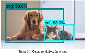Such in this case we can see that we have had two detected objects. One is Dog and another one is Cat. 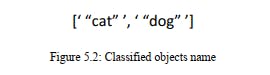We pass a picture to the organization, and it is then sent through different convolutions and pooling layers. At last, we get the yield as the article's class, genuinely direct. For each information picture, we get a comparing class as a yield. Would we be able to utilize this strategy to distinguish different articles in a picture? Indeed, we can! How about we take a gander at how we can take care of an overall article discovery issue utilizing a CNN. We first take a pre-prepared convolutional neural organization. Then, at that point, this model is retrained. We train the last layer of the organization dependent on the quantity of classes that should be distinguished. The third step is to get the Region of Interest for each picture. We then, at that point, reshape this large number of areas so they can coordinate with the CNN input size. In the wake of getting the areas, we train SVM to order articles and foundation. For each class, we train one double SVM. At last, we train a straight relapse model to produce more tight jumping encloses for each recognized item the picture. Here Dog, Cat is the class of those objects. we got detection score 98% for the Dog class and 88% for the Cat class. This isn’t end yet. We have the ultimate goal to announce those classes through voice pronunciation. 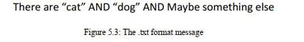A .txt format will travel through a function called text to speech function and ultimately the machine will give its generated voice output. TTS works with practically every close to home computerized gadget, including PCs, cell phones and tablets. A wide range of text records can be perused out loud, including Word and Pages reports. Indeed, even web-based website pages can be perused so anyone might hear. The voice in TTS is PC created, and perusing velocity can typically be accelerated or dialed back. Voice quality differs, however a few voices sound human. There are even PC created voices that sound like youngsters talking. Numerous TTS devices feature words as they are perused so anyone might hear. This permits children to see message and hear it simultaneously. There are two misfortune capacities we applied to both the RPN model and Classifier model. As we referenced previously, RPN model has two yields. One is for characterizing whether it's an article and the other one is for bounding boxes' directions relapse. From the figure underneath, we can see that it caught on quickly at the initial 20 epochs. Then, at that point, it turned out to be slower for classifier layer while the relapse layer actually continues to go down. The justification behind this may be that the exactness for objectiveness is now high for the beginning phase of our preparation, and yet, the precision of bounding boxes' directions is still low and needs more opportunity to learn. In this chapter we have showed result of Faster RCNN model. This model has already been pre-trained model. So, we have used this model for my convenience. This model worked very well for COCO dataset. We have got very good results using this model so we used this model in my dataset.

Chapter 6

Future Work & Conclusion

This chapter summarizes the whole research in several words describing the problem domain, previous researches, my contribution, experimental analysis and the outcomes of this research. Moreover, we have provided a brief study about the future scopes of this research.

6.1 Future Work

In future we will wish to add measurement feature such as how much the object is in size or how it locates etc. Passing on a road is difficult to move seamlessly. But this important feature is missing here. So, in future a deep action will be executed on this topic from us. we are also very keen to add a feature of GPS thus one can find out in real time where he is actually, will also help to take an alternative path for the user. Normally a blind people always need a guide to know that where he is. In the case of a big busy city or urban area it is very annoying to know the real time location of himself from the people. It is also sometimes time killing and confusing. So, this feature will add an extra comfort zone for the visual impaired people. A voice recommendation will be available in future thus it can suggest the user which path to choose. In a heavy traffic or industrial area, the traffic jam occurs regularly. In an emergency situation this is very frustrating to stuck with the traffic jam. This feature will be very time saving initiative for blind and normal people as well. We are planning an AI recommendation during road crossing. It is hard to find zebra crossing or green light signal for the blind people. So specific location the zebra crossing and the color of the signal light is very important feature. It will be a lifesaving initiative also.53 In Computer science image processing and computer vision is a rapid growing sector throughout the ages. So, there is no chance to be satisfied yet. With the time the demand is being raised dramatically. That’s why still we want to develop this project to the new functionalities. It was my very first work on image processing. So, with a limited knowledge of mine but tremendous support from my respected supervisor I got successfully done my work.

References

[1] “Digital image processing”, Rafael Gonzalez and Richard E. Woods, AddisonWesley, 2002

[2] World health organization, media center, visual impairment and blindness, fact sheet no.282,who.int/en/newsroom/factsheets/detail/blind..

[3] Anusha K V1, Devika K M2, Shrinidhi C Y3, Yashaswini M4, Dr. Madhu B K5 ,“ Navigation and Camera Reading System for Visually Impaired”, IRJET-2020

[4] Ashwani Kumar1, Ankush Chourasia2,“Blind Navigation System Using Artificial Intelligence”, IRJET-2018

[5] K. He, X. Zhang, S. Ren, and J. Sun. Deep residual learning for image recognition. In Proceedings of the IEEE conference on computer vision and pattern recognition, pages 770–778, 2016.

[6] J. Huang, V. Rathod, C. Sun, M. Zhu, A. Korattikara, A. Fathi, I. Fischer, Z. Wojna, Y. Song, S. Guadarrama, et al. Speed/accuracy trade-offs for modern convolutional object detectors.

[7] I. Krasin, T. Duerig, N. Alldrin, V. Ferrari, S. Abu-El-Haija, A. Kuznetsova, H. Rom, J. Uijlings, S. Popov, A. Veit, S. Belongie, V. Gomes, A. Gupta, C. Sun, G. Chechik, D. Cai, Z. Feng, D. Narayanan, and K. Murphy. Open images: A public dataset for large-scale multi-label and multi-class image classification.

[8] O. Russakovsky, L.-J. Li, and L. Fei-Fei. Best of both worlds: human-machine collaboration for object annotation. In Proceedings of the IEEE Conference on Computer Vision and Pattern Recognition, pages 2121–2131, 2015.

[9] Saurabh Gupta, Ross Girshick, Pablo Arbelaez and Jitendra Malik, Learning Rich Features from RGB- D Images for Object Detection and Segmentation (ECCV), 2014.

[10] Jizhong Xiao, Kevin Ramdath, Manor Iosilevish, Dharmdeo Sigh, and Anastasis Tsakas. A low-cost outdoor assistive navigation system for blind people. In Industrial Electronics and Applications (ICIEA), 2013 8th IEEE Conference on, pages 828–833. IEEE,2013.55

[11] Ross Girshick, Jeff Donahue, Trevor Darrell, and Jitendra Malik. Rich features hierarchies for accurate object detection and semantic segmentation. In Proceedings of the IEEE conference on computer vision and pattern recognition, pages 580–587, 2014.

[12] D. H. Ballard, “Generalizing the hough transform to detect arbitrary shapes," vol. 13, 1981, pp. 111-122.

[13] R. C. Bolles and R. A. Cain, “Recognizing and locating partially visible objects: The local-feature-focus method,” vol. 1, no. 3, 1982, pp. 57-82.

[14] D. Scherer, A. M¨uller, and S. Behnke, “Evaluation of pooling operations in convolutional architectures for object recognition,” pp. 92-101, 2010.

[15] N. Srivastava, G. Hinton, A. Krizhevsky, I. Sutskever, and R. Salakhutdinov, “Dropout: A simple way to prevent neural networks from overfitting," Journal of Machine Learning Research, vol. 15, pp. 1929-1958, 2014.

[16] C. Bishop, Springer Science Business Media, LLC, 233 Spring Street, New York, NY 10013, USA

[17] D. chen He and L. Wang, “Texture unit, texture spectrum, and texture analysis,” IEEE Transactions on Geoscience and Remote Sensing, vol. 28, no.4, pp. 509–512, July 1990.

[18] L. Bossard, M. Guillaumin, and L. Van Gool, “Food-101 – mining discriminative components with random forests,” in European Conference on Computer Vision, 2014.

[19] M. Liang and X. Hu, “Recurrent convolutional neural network for object recognition,” in 2015 IEEE Conference on Computer Vision and Pattern Recognition (CVPR), June 2015, pp. 3367-3375.

[20] Y. Li, X. Zhang, and D. Chen, “Csrnet: Dilated convolutional neural networks for understanding the highly congested scenes," CoRR, vol. abs/1802.10062, 2018.

[21] Ananth Noorithaya, M. Kishore Kumar, A. Sreedevi, “Voice assisted navigation system for the blind”, pp.256-257, 2014.

[22] Mounir Bousbia-Salah, Mohamed Fezari, “A Navigation Tool for Blind People”, chapter April, pp.333-337, 2007.56

[23] Harsha Gawari, Prof. Meeta Bakuli, “Voice and GPS Based Navigation System For Visually Impaired”, volume 4,pp.48-51,April 2014.

[24] W. K. Pratt, Digital Image Processing, New York: John Wiley & Sons, Inc., 1978.

[25] K. R. Castleman, Digital Image Processing, N. J., Englewood Cliffs: Prentice-Hall, Inc., 1979.

[26] R. C. Gonzales and P. Wintz, Digital Image Processing, Mass., Reading: AddisonWesley Publishing Company, Inc., 1977.

[27] C. Reader and L. Hubble, "Trends in image display systems", Proc. IEEE, vol. 69, no. 5, pp. 606-614, 1981

[28] E. L. Hall, "Almost uniform distribution for computer image enhancement", IEEE Trans. Computers, vol. C-23, pp. 207-209, 1974.

[29] H. C. Andrews, A. G. Tescher and R. P. Kruger, "Image processing by digital computer", IEEE Spectrum, vol. 9, no. 7, pp. 20-32, 1972.

[30] W. Frei, "Image enhancement by histogram hyperonization", Computer Graphics and Image Processing, vol. 6, no. 3, pp. 286-294, 1977.

[31] J. J. Sheppard, R. H. Stratton and C. Gazley, "Pseudocolor as means of image enhancement", Am. J. Optom. and Arch. Am. Ac. Optom., vol. 46, pp. 735-754, 1969.

[32] T. S. Huang, "Two-dimensional windows", IEEE Trans. Audio Electroacoustics, vol. AU-20, no. 1, pp. 88-89, 1972.

[33] R. M. Mersereau, W. F. G. Mecklenbräuker and T. F. Quatieri, "McClellan transformations for two-dimensional digital filtering: I-Design", IEEE Trans. Circuits Syst., vol. CAS-23, no. 7, pp. 405-414, 1976.

[34] B. R. Frieden, "A new restoring algorithm for the preferential enhancement of edge gradients", J. Opt. Soc. Am., vol. 66, pp. 3, 1976.

[35] T. S. Huang, G. T. Yang and G. Y. Tang, "A fast two-dimensional median filtering algorithm", IEEE Trans. Acoust. Speech Signal Processing, vol. ASSP-27, no. 1, pp. 13-18, 1979

[36] E. Ataman, V. K. Aatre and K. M. Wong, "A fast method for real-time median filtering", IEEE Trans. Acoust. Speech Signal Processing, vol. ASSP-18, no. 4, pp. 415-421, 198057

[37] J. Lee, "Digital image processing by use of local statistics", Proc. 1978 IEEE Computer Soc. Conf. on Pattern Recognition and Image Processing, pp. 55-61, 1978.

[38] R. E. Twogood and M. P. Ekstrom, "An extension of Eklundh's matrix transposition algorithm and its application in digital image processing", IEEE Trans. Computers, vol. C-25, pp. 950-952, 1976

[39] M. Onoe, "A method for computing large scale two-dimensional transform without transposing data matrix", Proc. IEEE, vol. 63, pp. 196-197, 1975.

[40] M. B. Ari, "On transposing large 2n×2n matrices", IEEE Trans. Computers, vol. C-27, pp. 72-75, 1979.

[41] A. K. Jain, "Image data compression: A review", Proc. IEEE, vol. 69, no. 3, pp. 349- 389, 1981.

[42] S. M. Pizer and A. E. Todd-Pokropek, "Improvement of scintigrams by computer processing", Seminars in Nuclear Medicine, vol. 8, no. 2, pp. 125-146, 1978.

[43] G. W. Wecksung and K. Campbell, "Digital image processing at E G & G", Comput., vol. 7, pp. 63-71, May 1974.

[44] Jing Min, "The application of digital image processing technology [J]", Mechanical management development, no. 01, 2011.

[45] Zheng Chanxiang, "Digital image processing technology and application of related research [J]", Digital technology and application, no. 09, 2013.

[46] He Dongxia, Li Zhulin and Wang jing, "Introduction to the application of digital image processing and the development tendency [J]", Journal of yanan university (natural science edition), no. 04, 2013.

[47] Zhang Junzhen, "Image segmentation method were reviewed [J]", Science and technology information, no. 06, 2012.

[48] Fan, Hongl, Li De-Minl, Liu TangYou and Cui Feng, "Using Interesting Examples for Teaching Digital Image Processing Course", Proceedings of 2009 4th International Conference on Computer Science and Education, pp. 1729-1732, 2009.

[49] Simon, Alejandrol, Adjouadi and Malek, "A programming tool for enhancing the teaching of image processing", Comput. Educ. J, vol. 17, pp. 85-94, 2007.

[50] Ning Yuan, Huang Runlin, Tan, Xin, Wei and Xuejun, "Research on the teaching reform of digital image processing course", Proceeding of International Conference on Educational and Information Technology, pp. 2457-2459, 2010.